Visualising data in Clojure with Hanami

At TPXimpact we publish a lot of data, but what can you do with a good dataset once it exists? In the previous post in this series, we learned how to download a dataset from the PMD open data platform; set up a Clojure programming environment, and create a new Clerk notebook. We left off with a working Clerk notebook and a preview of our data being rendered in a simple table (as shown above). In this post, we’ll learn how to use some tools from Clojure’s emerging data science ecosystem to visualise the data.

We’ll be taking advantage of Clerk’s built-in Vega viewer to render a Vega-lite specification to see our visualisation. We’ll also be using the Clojure library Hanami to help simplify writing the specification.

The code for the project as we left it is available on github. We’ll be building on top of where we left off in the first post.

Brief background on grammar for graphics

Before diving into the code again, it‘s helpful to have a basic understanding of how Vega approaches visualising data. Vega is a “grammar for graphics”, so it’s like a programming language but, rather than describing arbitrary instructions for a computer to execute, it describes what a data visualisation should look like in JSON. This is why it’s also commonly described as a “declarative” way to describe how to visually encode data and interactions into a format that can be rendered in a browser. We tell Vega what our visualisation should look like, and all of the details about how it gets rendered are left to the library. Like a language, we can think of Vega as being made up of words and rules for combining those words.

Vega-lite is built on top of Vega. It’s effectively a more concise version of the same library that abstracts away some of the details common to most visualisations. We’ll be working with Vega-lite for the rest of this tutorial.

The main components of the Vega-lite “language” are described below:

• data: input for the visualisation
• mark: shape/type of graphics to use
• encoding: mapping between data and marks
• transform: e.g. filter, aggregate, bin, etc.
• scale: meta-info about how the data should fit into the visualisation
• guides: legends, labels

These are some of the available JSON keys in a Vega-lite spec. The corresponding values are the “rules” for combining these “words”. Some examples are concat, layer, repeat, facet, resolve. There is more to Vega-lite, but this is enough to get started and to build the visualisation for our project. For many more examples of how this grammar is used to piece together “sentences” that Vega-lite can interpret and render as a graphic, see the Vega-lite website.

Rendering a Vega spec in Clerk

Now we can start exploring a bit in our notebook. As mentioned above, a Vega-lite spec is just some JSON data that uses specific, supported keys and values. Clojure can work with JSON, but conventionally uses EDN as a data transfer format. The “E” stands for “extensible”, so it supports more complex data structures than JSON does. This means that all JSON can be directly converted to EDN, but not the other way around. This is relevant because our Clerk notebook will expect Vega-lite specifications to be written in EDN, not JSON.

In order to get started, and see what Clerk does with a Vega spec, we can copy a simple example directly from the Vega-lite website. As an example, copy-pasting this Vega-lite specification for a visualisation of carbon dioxide in the atmosphere over time, into a JSON to EDN converter online gives us an EDN version of the specification.

For now, paste the EDN result into the notebook that we started last time. For a reminder about how to render the Clerk notebook in your browser, see the previous post. 

In annual_meal_temp_uk.clj:

Your copy-pasted EDN from the JSON conversion might appear more verbose, depending on how much whitespace is added for readability. Note that commas are optional in Clojure and they are interpreted as whitespace by the reader - exactly the same as spaces, tabs, and newlines.

To get Clerk to render this Vega-lite spec, we just need to pass it as the only argument to Clerk’s Vega viewer, clerk/vl, as in:

This won’t quite work yet, since the data source is specified as a relative path. To make it work we just need to update the value of :data > :url to a full URL: “https://vega.github.io/vega-lite/data/co2-concentration.csv"

This should render the visualisation in the notebook:

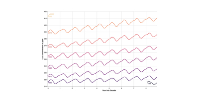
This spec is quite elaborate, but a useful demonstration of how all the components of Vega-lite come together to describe a data visualisation.

Hanami Setup

The next (and final) topic we’ll cover is Hanami. As you can see, Vega-lite specs can quickly become very verbose, so Hanami is a Clojure library that was developed to simplify writing these Vega specs. Using Hanami we can write compact, declarative, composable, and recursively parameterised visualisation templates.

The first step here is to add Hanami to our project. First we have to add it as a dependency and restart the REPL. Our deps.edn should look like this now:

In deps.edn:

Next, we require the relevant parts of Hanami in our notebook namespace declaration. We’ll be using Hanami’s commonand templates namespaces, so our namespace declaration should look like this:

In annual_meal_temp_uk.clj:

For the rest of this tutorial, it will be useful to have loaded and evaluated the notebook namespace in the REPL. In VSCode with Calva this can be done by opening the command palette and selecting “Calva: Switch Namespace in Output/REPL Window to Current Namespace” and then “Calva: Load/Evaluate Current File and its Requires/Dependencies”. This allows us access to all of these required namespaces directly from the REPL.

Hanami background

In Hanami, a “template” is just a Clojure map of substitution keys. The library defines many default substitution keys and a set of base templates to use as starting points, which you can see by entering @hc/_defaults in a REPL. This will print a big map with all of the default values that Hanami uses in the templates. By convention, Hanami substitution keys are all-caps symbols. To get the default value for a specific substitution key, Hanami includes a helper function hc/get-default. For example, to find the default value Hanami uses for all visualisation backgrounds, we can execute (hc/get-default :BACKGROUND) in the REPL, which returns"floralwhite".

The main function in Hanami is hc/xform. This is the transformation function that takes a template and optionally a series of extra transformation key/value pairs, inserting the values wherever the keys are specified in the template. If no key/value pairs are provided, Hanami uses the built-in defaults. To see what all this means, we can use Hanami to fill in a very basic template (remember, a template is just a Clojure map where the values are Hanami substitution keys. These are all-caps symbols, some of which have default values):

In the REPL (input> and output> are just prompts and will most likely be different in your REPL):

If we were to supply a custom value for :BACKGROUND, Hanami would use that instead, for example:

Transformations are recursive, i.e. the definitions of substitution keys can themselves contain substitution keys. For example, inspect the default value for :TOOLTIP:

The result includes several values which are themselves substitution keys. When used in a transformation and given no extra parameters, all of these values are replaced with the Hanami defaults:

If we supply any custom values to override these defaults, they will be used in the transformation:

This is a good time to note Hanami’s special “nothing” value, RMV. Notice in the above transformed :TOOLTIPexample that several of the keys that were specified in its definition have been removed. If you execute hc/RMV in the REPL, you'll see that it's just an alias for the special "nothing" value of the underlying library which Hanami uses for data manipulation (which is called Specter). If we check, for example, (hc/get-default :XTTITLE), we can see it's the same thing. This is a useful shortcut in Hanami to specify a default of "nothing" but to still include a given key in a template, which can be helpful to demonstrate to users which keys are available for writing generic, composable templates. Vega-lite does not gracefully ignore null values in specs, so we have to remove them before trying to render a visualisation.

The last relevant piece of background to understand in order to get started with Hanami is its built-in templates. The aerial.hanami.templates namespace defines several common Vega-lite chart templates and other useful composable chart components. See, for example, ht/bar-chart or ht/point-chart, by executing those statements in the REPL.

Putting it all together

We finally have all the necessary pieces to visualise our dataset from last time. To get started we can use Hanami’s built-in line-chart template. To render the skeleton of the chart, we can use Hanami to transform a bare-bones line chart template into a Vega-lite spec and tell Clerk to render it:

In annual_meal_temp_uk.clj:

Next, we need to supply our data to the graph. Vega-lite expects data to be in a tabular format, like a spreadsheet or database table. In JSON or EDN format this means the data looks like a collection of maps. Hanami will automatically convert data in CSV format to a vector of maps for us.

Hanami supports many different ways of specifying the data source. We can point Hanami to the data that’s already in a file in our project using the :FDATA substitution key (F for file):

We also need to tell Vega-lite which columns to use for the x and y axes:

This should be enough to get our data showing in our notebook!

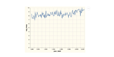
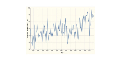
From here we can make some minor improvements. The effect of each extra value is explained in the comment beside it:

This tidies up our graph to something we can more easily interpret:

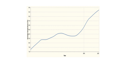
Vega-lite has many built-in transformations, including locally-estimated scatterplot smoothing, which can be used to produce a trend line. If we wanted to render a trend line, rather than plot each point individually, we just have to tell Vega-lite which axes to use in the transformation:

This will give us a smooth trendline, rather than a line connecting each point:

Vega-lite also supports layering two charts on the same set of axes, so we can layer these two graphs on top of each other to generate our final visualisation. Hanami includes a template to simplify this, ht/layer-chart. I’ve also changed the colour for the mark on the second graph by specifying a different value for :MCOLOR:

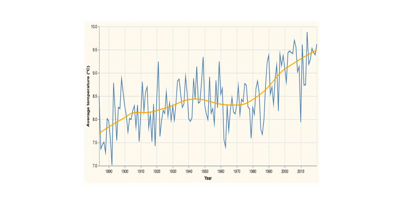
Conclusion

We have our Vega-lite spec being generated by Hanami and rendered with Clerk. Almost any visualisation you can imagine can be written as a Vega or Vega-lite specification, and Hanami also supports much more than we covered here. If you’re interested in learning more, both libraries have excellent documentation and lots of examples. The source code for this demo is also available on GitHub (the code up to this point is on the completed-visualisation branch). And, as always, feel free to reach out to me or the Clojure community in general wherever you find us on the internet.